What are RLC Circuits?

RLC circuits are electrical circuits in which resistors, inductors, and capacitors are connected either in series or in parallel. Their name derives from the symbols used to represent these elements in circuit diagrams, namely “R” for resistors, “L” for inductors, and “C” for capacitors.

Modern communication systems combine RLC circuits with active elements such as transistors and diodes to form complete integrated circuits. Within integrated circuits, RLC circuits function as filters, amplifiers, or oscillators, relying on characteristics such as resonance and damping to operate. In radio receivers, for example, RLC circuits perform band-pass filtering, allowing the user to tune into specific radio frequencies to the exclusion of others.

RLC circuits are also known as second-order circuits, arising from the fact that circuit designers use second-order differential equations to characterize the voltages and currents within these circuits. Furthermore, each R, L, and C element within these circuits can be arranged in a number of different topologies, with the simplest being series and parallel topologies.

Within pure RL and RC circuits, only one energy storage element is present in the form of an inductor (L) or a capacitor (C). In both these cases, circuit designers need only specify one initial condition, resulting in first-order differential equations.

In contrast, RLC circuits contain both energy storage elements, thereby requiring two initial conditions and resulting in second-order differential equations. These initial conditions pertain to the initial voltages and currents present in the circuit.

It’s also worth noting that, up until the beginning of the 20th century, second-order differential equations were thought to provide a complete description of the behaviors of physical systems. However, with the efforts of Max Planck in formulating the principles behind quantum mechanics, this view has now changed.

Nonetheless, second-order differential equations continue to provide accurate descriptions of the behaviors of many physical systems. One example is the swinging of a pendulum, in which potential energy in the gravity field is transformed into kinetic energy as the pendulum is released, which is then transformed back into potential energy as it reaches its maximum height. As the pendulum dissipates energy (due to friction), it gradually comes to rest.

As it happens, second-order differential equations provide accurate descriptions of systems in which there is a periodic exchange of energies, as illustrated in the pendulum system. This periodic energy exchange mirrors the behaviors of RLC circuits, in which there is a periodic interchange between electrical and magnetic energy fields.

RLC circuits incorporating resistors, inductors, and capacitors form the foundation of electric circuit design. Each of these elements exhibits specific physical characteristics that contribute to overall circuit behavior.

Resistors

Resistors are lumped circuit elements that “resist” the flow of currents, thereby causing a drop in voltage. They’re characterized by a constant resistance (measured in ohms) that is independent of the frequency of an applied signal. Resistors are indispensable in maintaining an equilibrium within an RLC circuit.

Inductors

Inductors are typically constructed from coils of wire, storing energy in a magnetic field as current passes through the wire. They oppose variations in current, where the degree of opposition is known as the inductive reactance (measured in ohms). This inductive reactance is dependent on the frequency of an applied signal. It increases as frequency increases, and vice versa.

Capacitors

Where inductors store energy in a magnetic field, capacitors store energy in an electric field. Capacitors oppose variations in voltage where the degree of opposition is known as the capacitive reactance (also measured in ohms). The capacitive reactance is also frequency dependent: It decreases with increasing frequency, and vice versa.

RLC circuits comprise two main components, power sources and resonators. Further, there are two types of power sources — Thévenin and Norton power sources — and also two types of resonators — series LC and parallel LC resonators. Series and parallel RLC circuits each exhibit distinct characteristics, making each suitable for specific applications.

Characteristics of Series RLC Circuits

In a series RLC circuit, resistors, inductances, and capacitors are arranged on a single circuit path, such that the current flowing through each component remains unchanged while the voltages vary. The net effect is that:

• Across a resistor, the voltage is in phase with the current.
• Across an inductor, the voltage leads the current by 90°.
• Across a capacitor, the voltage lags the current by 90°.

As a consequence, the total voltage across the circuit is not the algebraic sum of the voltages across each component, but rather their vector sum. These voltages can be plotted on a phasor diagram, using the current vector for reference.

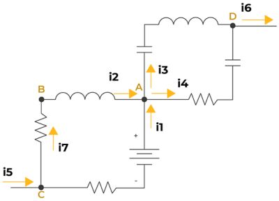
Kirchhoff’s Voltage Law (KVL) states that the sum of the voltages in a closed circuit equals the sum of the electromotive forces (EMFs) across this circuit. Therefore, the source voltage VS (in volts) is:

VS = VR + VL + VC

Given that, in a series RLC circuit:

VR = IR

VL = LdI/dt

VC = Q/C

This becomes:

VS = IR + LdI/dt + Q/C

Where I is a current, L an inductance, Q an electrical charge, and C a capacitance.

Any circuit naturally imposes a certain degree of resistance to the flow of current. This is known as the impedance (in ohms). It comprises a “resistive” part (resistance to direct current flow) and a “reactive” part (resistance to alternating current flow). In a series RLC circuit, it is expressed as:

Z = √R2 + (XL2 - XC2)

Where XL is the inductive reactance (opposition to alternating current flow at the inductor) and XC is the capacitive reactance (opposition to alternating voltage at the capacitor).

Inductive and capacitive reactances are both frequency dependent, such that: 

• When XL > XC the overall reactance in the circuit becomes inductive, and the voltage leads the current by a 90° phase angle. 
• When XL < XC, the circuit becomes capacitive, and the voltage lags the current by 90°.  
• When XL = XC, the circuit becomes resonant. This has a number of important applications in electronic circuits.

Characteristics of Parallel RLC Circuits

In a parallel RLC circuit, the voltage remains the same across the R, L, and C components while the current flowing through each component can vary. A parallel RLC circuit is the reciprocal of a series circuit; however, its mathematical treatment is more challenging.

The total current flowing through the circuit does not equal the algebraic sum of the currents flowing through each element, but rather their vector sum.

Kirchhoff’s Current Law (KCL) states that the sum of the currents flowing through a node in a circuit equals zero. Therefore, the source current at any node in the circuit is given by:

IS - IR - IL - IC = 0

And the impedance is:

1/Z = √(1/R)2 + (1/XL - 1/XC)2

It’s worth noting that the above expression is the reciprocal of the equation for the impedance in a series RLC circuit. In fact, because of the duality relationship that exists in electrical circuits, the properties of a parallel RLC mirror those of a series RLC. Consequently, the impedance for a parallel RLC is the dual of a series RLC, and the expressions adopt the same general form.

The reciprocal for the impedance (1/Z) is called the admittance (measured in siemens). It presents a more convenient way to calculate impedances in parallel circuits, especially where several branches are involved. The total admittance in parallel circuits is simply the sum of the elemental admittances. Reciprocally, in series circuits, the total impedance is the sum of the elemental impedances.

As a point of interest, the reciprocal of the resistance (1/R) is known as the conductance, and the reciprocal of the reactance (1/X) is known as the susceptance.

Differences Between Series and Parallel RLC Circuits

As previously discussed, the circuit expressions for the series and parallel configurations are the inverses of each other. This helps circuit designers determine whether a series or parallel configuration is more convenient for a particular design. The following tables describes the key differences between series and parallel RLC circuits:

Fundamentally, there are two parameters describing the behavior of RLC circuits, namely the resonance frequency and the damping factor. Engineers may derive other parameters, including bandwidth and Q-factor, from these first two.

Resonance in RLC Circuits

An important characteristic of RLC circuits is the ability to resonate at specific frequencies, known as the resonant frequencies. Physical systems exhibit natural frequencies at which they vibrate more readily. At resonance (either in the presence or absence of a driving source), vibrations are greatly amplified, resulting in efficient energy transfers.

Within an RLC circuit, the energy stored in a capacitor’s electrical field may be transferred and stored into the magnetic field surrounding an inductor, and vice versa. This transfer may occur periodically, resulting in an oscillating RLC circuit. At resonance, the angular frequency ω (in radians) is given by:

ω = 1/√LC

Also, at resonance, the inductive reactance equals the capacitive reactance, and the total impedance of the circuit (a complex number) is zero.

Consequently, in a series RLC circuit, impedance reaches a minimum, whereas it reaches a maximum in a parallel circuit. 

Understanding and applying resonance in RLC circuits is crucial for designing efficient and effective electronic systems, particularly in communications, power systems, and signal processing applications. Important resonance applications include:

• Frequency selection: At resonance, RLC circuits can respond to signals of specific frequencies to the exclusion of other frequencies — for example, the tuner in a radio.
• Filtering: RLC circuits can function as various types of filters, including band-pass, band-stop, low-pass, or high-pass filters. Alternatively, these circuits can function as noise filters in integrated circuits. They can also function as rejector circuits, suppressing currents at specific frequencies, and this type of parallel circuit is known as an antiresonator.
• Voltage multiplication: If the resistance is minimal, the voltages across the inductor and capacitor can be several times larger than the input voltage. This voltage multiplication effect is proportional to the circuit's Q-factor.
• Impedance matching: At resonance, the impedance in a series RLC circuit is purely resistive and at its minimum, while for a parallel RLC circuit, it is at its maximum. This can be used for impedance matching.
• Power transfer: As series RLC circuits reach maximum power transfer at resonance, they’re pivotal to applications requiring efficient energy transfer.
• Oscillator circuits: RLC circuits are commonly used in oscillator applications, where sustained oscillations at a specific frequency are required. In these instances, the circuit's resistance is minimized (for series circuits) or maximized (for parallel circuits) to reduce damping and approximate an ideal LC circuit.

Damping in RLC Circuits

Damping describes the tendency in oscillating RLC systems for oscillation amplitudes to decrease over time (due to resistances). Therefore, resistors play a crucial role in dissipating energy within RLC circuits. They also determine whether the circuit will resonate naturally (that is, in the absence of a driving source).

Thus, engineers observe three types of damping responses within RLC circuits:

• Underdamped circuits, characterized by a slow decay in oscillations
• Overdamped circuits, where oscillations cease quickly
• Critically damped circuits, where oscillations cease just short of the critical time needed to reach steady state oscillations
• For critically damped circuits, \zeta = 1

The dimensionless damping ratio is an important parameter that helps engineers characterize damping in RLC circuits. In oscillator circuits, engineers seek to minimize damping by minimizing the resistance in a series circuit while maximizing the resistance in a parallel circuit. In band-pass filters, the damping coefficient is tuned to match the desired bandwidth: A higher value results in a wider bandwidth and vice versa.

Derived parameters in RLC circuits include bandwidth and Q-factor.

Bandwidth

The bandwidth describes the range of frequencies at which an RLC circuit resonates. It represents a key parameter in filter design, in which a rapid change in impedance near resonance can be used to pass or block signals close to the resonance frequency — an effect apparent in band-pass and band-stop filters, respectively.

Bandwidth represents the frequency gap between the cut-off frequencies, typically defined as the frequencies at which the power passing through the circuit is half the power passing at resonance. 

Engineers tune the damping in filter circuits to match the desired bandwidth. High damping results in a wide-band filter. Conversely, low damping results in a narrow-band filter.

Q-factor

The dimensionless Q-factor describes how much an oscillating system is damped. It is defined as the ratio of the initial energy stored in the system to the energy lost in one radian of an oscillation cycle.

A higher Q-factor represents a lower rate of energy loss with oscillations dying out more slowly (narrow-band, underdamped), while a lower Q-factor represents a lossy network (wide-band, overdamped). Examples of high-Q systems include clocks, lasers, and tuning forks, the latter displaying a Q in the region of 1000. Some high-Q lasers reach Q values of 1011 or higher.

RLC circuits that integrate resistors, inductors, and capacitors form the backbone of circuit design. Leveraging circuit characteristics of resonance and damping, engineers can design a variety of circuits for use in a range of applications. Therefore, understanding and characterizing RLC circuits is crucial to the design, analysis, and optimization of circuits that are assimilated to a variety of electronics and communications systems.

Within RLC circuits, electromagnetic coupling is a critical factor impacting the performance of these circuits — affecting frequency response, power transfer, damping, and other characteristics.

For this reason, concerning circuit design, Ansys Exalto ® software is a post-LVS RLCk extraction software that empowers designers to accurately capture crosstalk among different blocks in the design hierarchy by extracting lumped-element parasitics and generating an accurate model for electrical, magnetic, and substrate coupling. Exalto software interfaces with most LVS packages and complements the RC extraction tool of choice.

In addition, Ansys RaptorH ™ software is a pre-LVS electromagnetic modeling software allowing for the high-capacity electromagnetic modeling of high-speed RF and digital SOCs, including power grids, full custom blocks, spiral inductors, and clock trees. It combines the gold-standard Ansys HFSS™ electromagnetic simulation engine with the silicon-optimized Ansys RaptorX engine.

Related Resources