What is Turbulent Flow?

A defining characteristic of fluids is that they are not rigid but flow in and around solid objects. Turbulent flow occurs when the particles in the fluid start to move perpendicular to the dominant or mean flow direction and exhibit chaotic changes in direction, flow velocity, and pressure. This perpendicular, often circular movement is referred to as an eddy or swirl. This is in contrast to laminar flow, in which the particles move parallel to one another. 

Laminar flow transitions to turbulent flow when the inertial forces created by the kinetic energy of the liquid or gas exceed the viscous forces of the fluid. Turbulent flow is chaotic and can’t be defined with a deterministic set of equations. Instead, engineers use statistical methods to predict highly irregular behavior. 

Because of the chaotic nature of turbulent flow, the science of fluid mechanics uses statistical methods to characterize and predict fluid velocity, velocity fluctuations, and pressure fluctuations caused by turbulent flow. This characterization starts with the dimensionless quantity called the Reynolds number. Further equations then capture other behaviors useful in designing or accounting for turbulent flow.

Predicting Turbulent Flow: Reynolds Numbers

In 1883, Osborne Reynolds published a paper describing the transition from laminar to turbulent flow in a simple pipe. The data showed how the ratio between internal and viscous forces predicts how likely it is for turbulence to occur. This dimensionless value is referred to as the Reynolds number.

The equation to determine the Reynolds number is:

In general, flows with low Reynolds numbers stay as laminar flow because they lack the kinetic energy needed to convert any instabilities in the fluid motion into flow perpendicular to the mean flow direction. As the flow velocity or density increases relative to the viscosity of the flow, turbulence is more likely. 

4 Important Characteristics of Turbulent Flow

Other important characteristics of turbulent flow that engineers, physicists, and chemists must take into consideration are: 

1. Fluctuations and Eddies

An important measure of turbulent flow is fluctuation — the variation in velocity in magnitude and direction from the mean velocity magnitude and direction. When fluctuations exhibit a swirling, circular motion, they are called eddies. These variations in flow drive the velocity vector pressure and temperature of the fluid, as well as the kinetic energy and mixing in chemical reactions and the shear loads on structures. 

2. Dissipation

The kinetic energy that creates turbulent flow is converted into internal energy through viscous shear stress. The energy in large eddies cascades into smaller eddies with more shear forces, and these cascade into ever smaller eddies with increasing shear forces. As the eddies get smaller, the kinetic energy dissipates as viscous energy. 

3. Kinematic Energy and Viscous Energy

The kinematic energy in turbulent flow is the amount of kinetic energy per unit volume, and it represents the average energy of the turbulent velocity fluctuations in the flow. The viscous forces in the fluid convert some of the kinetic energy into heat due to internal friction. The amount of heat converted is called the viscous energy. 

4. Mass, Momentum, and Energy Transport

Any engineer or scientist working with fluid dynamics wants to know how mass, momentum, and energy transfer within the fluid flow they are studying. This is especially important in turbulent flow because it impacts the rate of all transport behavior. This transport can also be referred to as turbulent diffusion. 

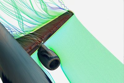
Engineers use computational fluid dynamics (CFD) to predict the behavior of turbulent flow. This numerical method breaks a flow regime up into cells and calculates the velocity, pressure, density, and temperature in each cell using the governing equations for the conservation of energy, mass, and momentum in fluids. 

CFD software solutions like Ansys Fluent fluid simulation software and Ansys CFX CFD software predict turbulence by first determining when a flow transitions from laminar to turbulent. Where turbulent flow exists, the solvers use a variety of simplified equations to calculate the velocity, pressure, temperature, and vorticity caused by turbulent flow. 

Engineers can conduct relatively simple flow simulations of mixing different materials or extremely complex multiphysics models that include the impact of both laminar and turbulent flow on optical, thermal, and structural performance. Before selecting a turbulence model, the keys to success are accurately capturing the geometry, establishing the correct boundary conditions and constraints, defining the material properties, and applying the proper mathematical models. When engineers need to predict turbulent flow, those models usually consist of two classes of simplified equations.

Reynolds-averaged Navier-Stokes (RANS) Models for Turbulence

The first class of turbulence modeling equations are RANS models. This approach decomposes flow quantities into the mean flow and fluctuating components. RANS models use empirical studies to approximate turbulent behavior. Some of the more commonly used RANS models are:

• Spalart-Almaras (SA) model: A simple model that solves a single transport equation. It is commonly used for external flow, especially in aerodynamics, and is a low-Reynolds number model. 
• Two-equation models: Engineers use a family of models that use two transport equations. Two equations allow for the modeling of history effects like the diffusion of turbulent energy and convection. The first transport variable determines the kinetic energy in the turbulence, and the second transport variable represents the length or time scale of the turbulence. Common two-equation models include generalized k-⍵ (GEKO), baseline (BSL), shear stress transport (SST), and K-epsilon (k-ε). These models can be used independently or combined. They are most often used for industrial applications. 

Scale-resolving Simulation Models for Turbulence

The second class of turbulence modeling, scale-resolving simulation, does not average turbulent fluid flow over time. Instead, it solves for turbulent fluid flow over time and space. Most applications of SRS use large eddy simulation (LES) models to solve for larger eddies while modeling the smaller eddies separately. 

LES models have been improved and validated over some time. However, because they require longer solve times and larger numerical models, they were not used as frequently until recent improvements in computer performance were made. LES models require more cells and longer run times compared to RANS models. The increase in computing capability, especially the use of GPUs, enables the use of SRS models for industrial flows with a variety of SRS/RANS hybrid models, including:

• scale-adaptive simulation (SAS)
• detached eddy Simulation (DES)
• shielded detached eddy simulation (SDES)
• stress-blended eddy simulation (SBES)
• embedded LES (ELES)

From blood flow in your body to the cooling of your computer and airplanes flying through the air, turbulent flow impacts how fluids move through a system and how it interacts with the solids it touches, as well as chemical reactions and heat transfer. Some designs are optimized to maintain laminar flow and avoid turbulent flow. In other situations, there are benefits to turbulent flow. Engineers and scientists study fluid dynamics to understand turbulent flow so they can manage it and take its effects into account in their designs. 

One important characteristic of turbulent flow is that it increases the mixing of a fluid. This mass transport increases diffusion rates, speeds up chemical reactions, and increases heat transfer into and within the fluid. In the combustion and cooling of gas turbines, turbulent flow is encouraged to achieve more efficient combustion and improve the internal cooling within turbine blades. Mixing applications also use turbulence to speed up the combination of materials or dissolve particles faster. 

Blood flow is a good example of how turbulent flow can cause problems. The shear stresses caused by eddies in blood can result in thrombosis, forming clots in the blood that can block flow. An important part of aerodynamic design is reducing drag by using turbulence to delay flow separation by allowing turbulence in areas of adverse pressure gradients and reducing turbulence where it increases drag. Large vortices caused by turbulence can also create noise or exert pressure loads on structures. Engineers designing buildings and bridges account for the pressure loading caused by eddies generated in turbulent wind flow around the structure. 

Explore the Ansys Fluids collection to learn more.

Related Resources